16 |
Oilfield Technology
June
2016
and successfully deployed them as a coherent
means by which effective, tailored geophysical
solutions are delivered. This article describes
the implementation of XArray, the technical
background behind the method and component
technologies, and gives insight into some field
examples.
With ever increasing pressure on E&P company
budgets and often tight timelines to get from first
shot to interpretable product, streamer spread
dimensions have grown in size to achieve greater
coverage per vessel pass while maintaining the
trace density required to meet the geophysical
objectives of the survey. On the data quality
side, streamers themselves have gotten longer,
targeting deeper reflectors while improving
S/N gained from higher fold. Recording systems
have in turn grown in capacity to keep pace with
these increases in the size of towed receiver
arrays, however the introduction of continuous
recording functionality would arguably have just
as significant an impact on the volume of data
recorded per unit survey area and, by extension,
acquisition efficiency and data density.
To demonstrate this, it is worth considering
the limitations to the data acquisition process
presented by the absence of continuous recording.
Data acquired without using continuous
recording is often referred to as being source
initiation constrained, where the time between
shots must be greater than the fixed record
length for recording of that shot to occur. Thus
deeper targets (longer record lengths) required
sufficiently spaced shotpoint intervals to
ensure that there was enough time between
shots to capture the pre-set record length. As
a result shotpoint interval/record length pairs
of 18.75 m/7 seconds; 25 m/10 seconds; and
37.5 m/13 seconds in the case of wide azimuth
acquisition became industry standard based on
nominal vessel speeds. The advent of continuous
recording however, enabled the decoupling
of the frequency of source initiation from the
record length captured. Firing several shots in
the timeframe required to capture any one of the
associated shot records is now entirely possible,
making the standard shotpoint interval/record
length pairs largely irrelevant from the perspective
of what is technically achievable in acquisition. As
an example, Polarcus recently acquired a survey
where a source fired on average every 3 seconds
with a 10 second record length delivered from each
shot location.
Being able to fire as frequently as needed
and capture records of lengths as needed does
not tell the full story. The physics suggests that
increased shot frequency would also result in
shallow reflections from subsequent shots being
superimposed on deeper reflections from earlier
shots. This phenomenon highlights the second
crucial component technology of XArray, which is
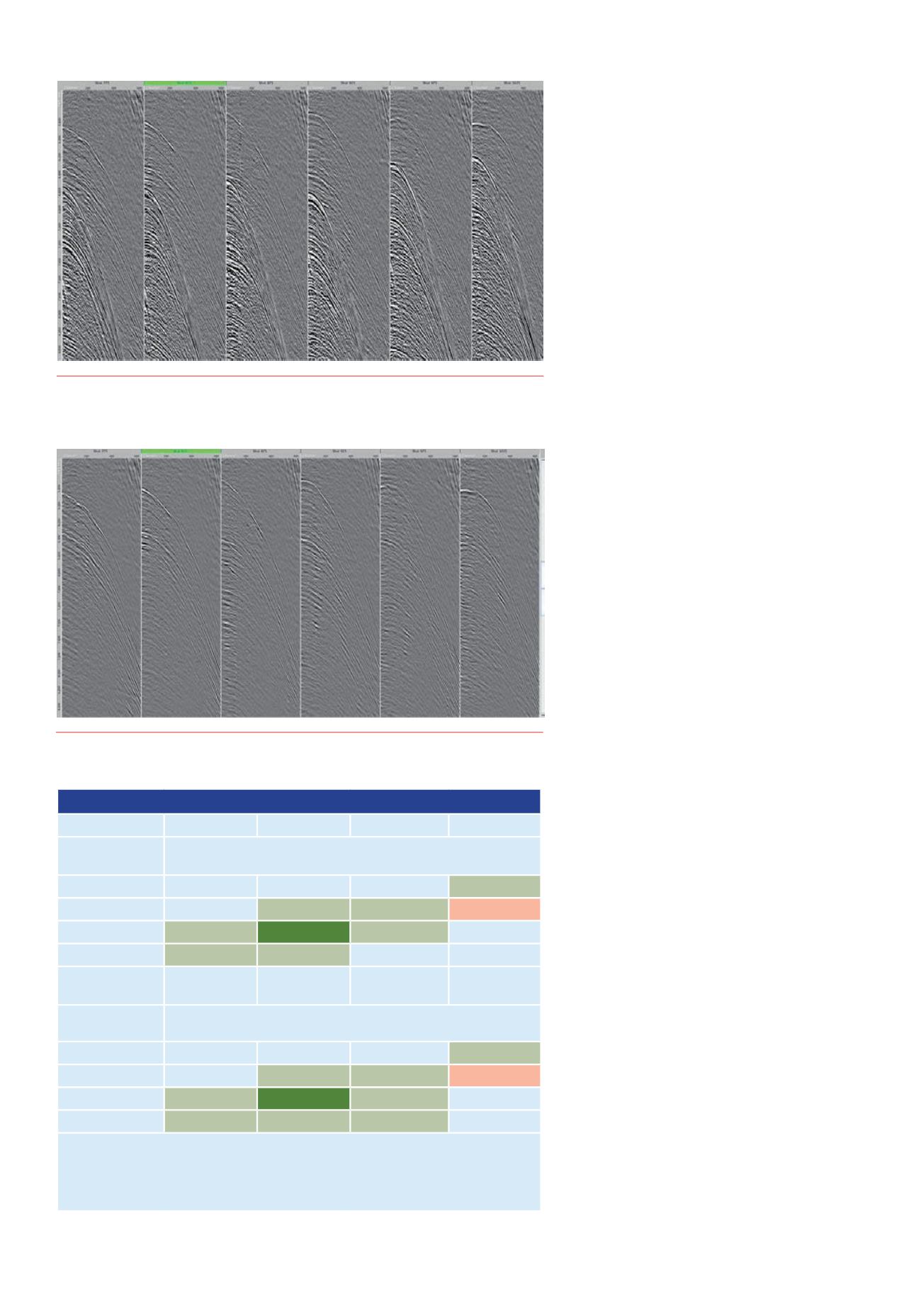
Figure 2.
Shotput record shown in Figure 1 after removal of overlapping shot.
Figure 1.
Shot record fromthe Capreolus 3D survey showing overlapping shot energy
startingat 6 seconds (12.5mSPI).
Table 1. Subsurface line shotput interval and nominal fold
Sail line SPI (m)
10
12.5
18.75
25
Number of
sources
Subsurface line shotput interval (m)
1
10
12.5
18.75
25
2
20
25
37.5
50
3
30
37.5
56.25
75
5
50
62.5
93.75
125
Number of
sources
CMP fold achieved with 8 km streamers
1
400
320
213
160
2
200
160
106
80
3
133
106
71
53
5
80
64
42
32
The table shows subsurface line shotput interval and nominal fold for different combinations
of sail line shotput and number of sources. Cells highlighted in light green refer to typical
configurations found in conventional and XArray acquisition. Dark green and orange cells
compare an example XArray triple source configuration, and a conventional dual source
configuration respectively.


