18 |
Oilfield Technology
May
2016
should raise a red flag regarding the reliability of the velocity
model. Figure 1 illustrates this concept in two different geological
settings: salt regimes and fault systems. The figures portray the
expected distortions in cases where the velocity model is not
accurate, and the respective structures with the correct velocity
model:
Ì
Salt body:
If the salt body is filled with high constant salt
velocity without taking into account the change of velocities
due to intrusions, the salt base and seismic events below will
present a deformation, indicated by a pull-down. If the velocity
model takes into account such an intrusion, the salt base and
structure beneath are properly located in depth, removing the
pull-down effect (Figure 1a).
Ì
Fault shadow:
The observed pull-up beneath the fault structure
suggests that the velocity contrast between the layers and the
fault positioning is not properly resolved. If the fault positioning
and velocity contrast are correctly mapped, the fault shadow
effect beneath fault structures does not impact the seismic
image (Figure 1b).
Methodology
Ray-based reflection tomography is used to globally update the
background model in depth (axial velocity, Epsilon and Delta) using
depth migrated gathers.
3
The goal is to associate changes in the
model parameters (e.g. axial interval velocity, Thomsen anisotropy
interval parameters, and reflectors’ depth) along ray pairs to travel
time errors computed from residual moveouts along migrated
gathers, through global minimisation in which a set of linear
equations is solved.
In the case of mistie or welltie tomography, migrated gathers
have already been flattened; therefore, travel time errors along
the ray path are equal to zero. Equation 1 describes the linear
relation between changes in the model parameters along ray pairs
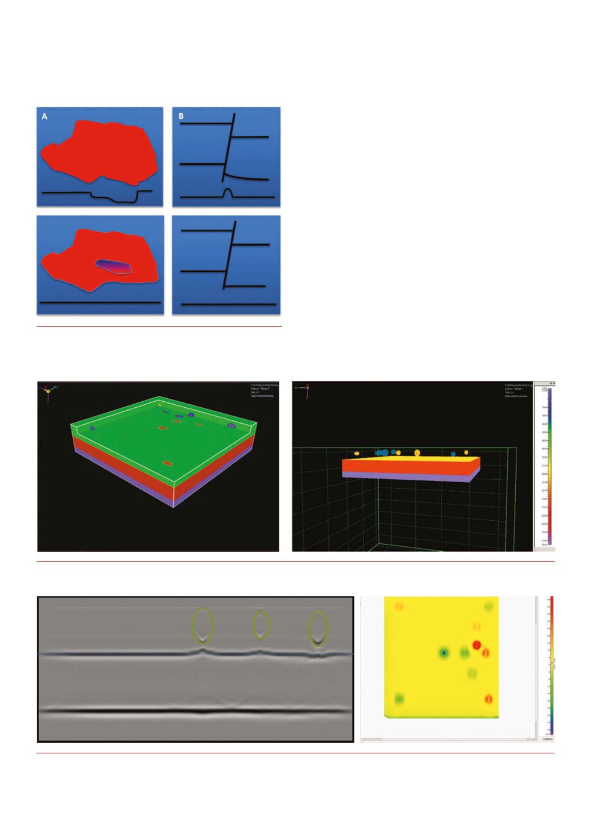
Figure 1.
Top images illustrate questionable geological scenarios in
a salt regime (left) and fault system(right). Bottomfigures portray the
expectedgeological scenarioswith the correct velocitymodel (salt – left,
fault – right).
Figure 2.
Original velocitymodel used formodelling. Left – volume viewed fromabove showinga slice at 250mthat cuts different lenses. Right – viewed
fromthe side, showing lenses in upper 600m.
Figure 3.
Display of the seismicmigrated section using the altered velocitymodel. Pull-ups andpull-downs are visible. Overlaying the seismic event inblue
is the expected interpretation; the current interpretation is ingreen (left). Mistiemap computedby subtracting current fromsuspected interpretation.
C
M
Y
CM
MY
CY
CMY
K


