26 |
Oilfield Technology
May
2016
Constructionoftheper-faciesLFMs
In its simplest form, impedance log data can be plotted as a
function of depth below an appropriate datum restricted to a
particular facies, and then fit a compaction curve to that data,
complete with an assessment of uncertainty. In 3D, it is possible
to take the horizon representing the datum and ‘hang’ the
compaction curve off that horizon at all trace locations. Again
uncertainty is incorporated. Figure 2 shows an example of this
process.
For a review of promising alternative approaches see
Hansford et. al. (2016).
3
The crux of this article is that geologists
cannot assist the geophysicist sensibly in the construction
of one LFM that needs to represent all facies (as in model
based inversion to date), but that they can help greatly in the
construction of e.g. a carbonate-only LFM, a sand-only LFM, etc.
Casestudy
Ikon Science applied both facies-agnostic model-based inversion
and the new facies-aware models-based inversion to the
2700 km
2
Willem 3D seismic survey within the Carnarvon basin,
North West Shelf, Australia. Interpreted horizons were available
for key events.
Within the study area there are six wells. Five of these wells
had logs (but of those only two wells had a complete suite
of elastic logs), and for the remaining well, Pyxis-1, only the
location and the fact that it was a gas discovery were known.
For the facies-aware models-based inversion five elastically
distinct facies were first identified: shale, marl, limestone, brine
sand and gas sand. After making impedance depth trends for
these five facies using the top of the Cretaceous as a datum, five
simple LFMs were constructed, by ‘hanging’ the depth trends
from the top Cretaceous horizon. The result of this facies-aware
models-based inversion is presented in Figure 3.
Against the company’s better judgement (as only five
wells undersamples an area of 2700 km
2
hugely in case of well
log interpolation) it created one LFM using the horizons as a
guide in the impedance logs interpolation, and subsequently
ran classical model-based inversion. As this only results in
impedances, a Bayesian Classification (Sams & Saussus, 2010)
4
was subsequently performed to obtain a facies image (same five
facies as used earlier). The result is presented in Figure 3.
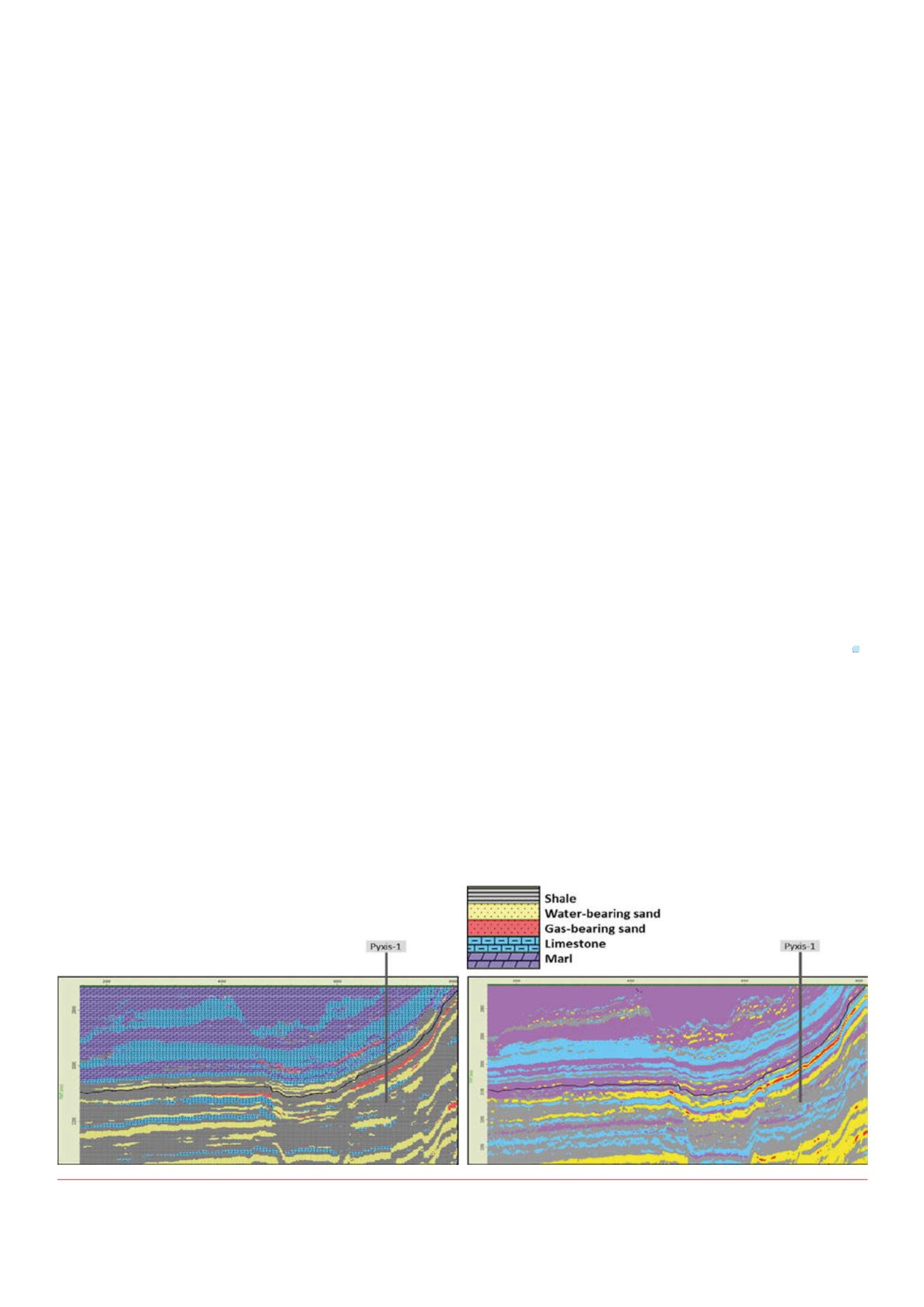
Inspection of Figure 3 shows that incorporation of facies
within the seismic inversion makes a big difference:
Ì
Ì
A clear gas column is seen at the Pyxis-1 well; 18.3 m was
the original prediction; this compares very favourably
to the 19.5 m gas column announced by the operator,
Woodside (note that the imaging of the gas column in case of
facies-agnostic model-based inversion is poorer, with brine
sand either side of the gas sand).
Ì
Ì
Although perhaps not economically viable, to the west of
the Pyxis-1 well a thin gas accumulation is imaged, with a
beautiful gas-water contract (note that this thin gas column
is absent in case of facies-agnostic model-based inversion).
This case study is explained in more detail in Sams et. al. (2016).
5
Conclusions
This article has shown that in seismic forward modelling, rock
facies constitutes a key component but that in model-based
seismic inversion (where seismic forward modelling takes place
repeatedly in the optimisation loop) facies is absent. This is
an odd state of affairs and so Ikon Sciences introduced a new
seismic inversion methodology where facies are incorporated.
The key difference is that, whereas in facies-agnostic
model-based inversion to date the company specify one LFM of
impedances that needs to represent all facies (even though prior
to inversion it is not known where these facies are located in the
subsurface), in the new facies-aware models-based inversion,
multiple easy-to-construct LFMs are specified, one per facies
expected, and then the inversion determines the one LFM it
ultimately uses.
The case study shows that this quite simple idea of
overspecifying the low frequency information gives a much
improved facies image of the subsurface, which can be used to
good effect in prospect generation and analysis, development and
production geological modelling (and on to flow simulation etc.).
References
1.
Wideness, M.B., ‘How thin is a thin bed?’,
Geophysics
, 38, (1973),
pp. 1176 - 1180.
2.
Kemper, M. and Gunning, J., ‘Joint Impedance and Facies Inversion –
Seismic inversion redefined’,
First Break
, 32, (2014), pp. 89 - 95.
3.
Hansford, J., Kemper, M., Abel, M. and re Ros, L.F., ‘Integration of
lithological data for advanced seismic inversion’, EAGE/SBGf lacustrine
carbonate workshop, Rio de Janeiro, (2016).
4.
Sams, M. and Saussus, D., ‘Uncertainties in the quantitative interpretation
of lithology probability volumes’,
The Leading Edge,
(2010).
5.
Sams, M., Westlake, S., Thorp, J. and Zadeh, E., ‘Wllem 3D: reprocessed,
inverted, revitalised’,
The Leading Edge
, V35, N, (2016).
Figure 3.
Faciesmodel fromfacies-awaremodels-based inversion (left) and fromfacies-agnosticmodel-based inversion (right). With thanks to Searcher
Seismic and SpectrumMulti-client for allowingaccess to the dataandpermission to publish.


