identified further adjustments and refinement to the model
is made.
Secondly, smaller pipeline sections are defined and
the coating resistance of each section of the individual
pipelines is adjusted until the simulation results are aligned
with accurately measured field data. Persistent deviations
are often explained by incorrect or missing field data and
undocumented changes to the system. Typical examples
are accidental drains, failed equipment or non-reported
bonds or electrical shorting. Once clarified a baseline
model with the correct distribution of the CP current is
obtained. Multiple iterations and a continual integration
of field data are required to obtain a realistic model of
such a complex system. Some special algorithms are under
development to automate this process.
Finally, the model allows a quantitative analysis of the
CP effectiveness, where the OFF potential and coupon
current demand are used to define the polarisation curve
of steel in the local soil. Since the CP current distribution
has been calculated for each pipeline section in the
previous step, the amount of current entering the pipe
through the soil is now known. Through the polarisation
curve, the current can then be converted to true or IR-free
potential of the pipeline. Polarisation levels can be further
refined by characterising the size and amount of coating
defects. Segments that do not receive sufficient CP current
or experience an anodic stress due to the other pipelines
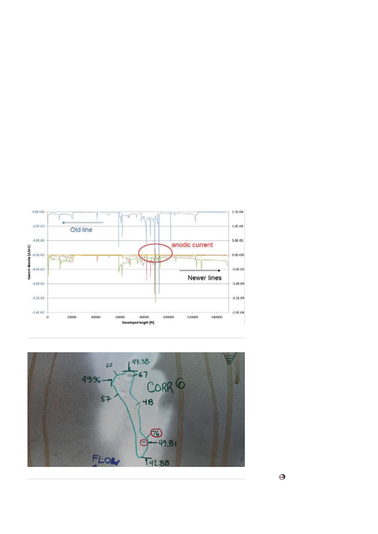
present in the same ROW become apparent. As an example,
Figure 4 shows an area with a transition of soil type near
a waterway that resulted in some sections on two recent
pipelines tending to have (slightly) positive or anodic
current density.
Treat the disease, not the symptoms
Once the model is in place, strategic counter measure
scenarios can be reviewed at the design stages of
expansion projects for a relatively low cost. Ad hoc actions
in the field such as adding anode beds to bring potentials
to more negative values can sometimes worsen the
situation in unexpected remote locations. Equipotential
bonds should be installed at the
appropriate locations to avoid CP
currents from flowing in undesirable
directions.
Alternatively, the model has
revealed that it is crucial for shunt
resistors to be installed for each
rectifier negative cable connecting
the individual pipelines. The value of
the resistor is calculated by dividing
the average IR-free potential by the
axial current occurring in the sections
with the most electropositive
potentials. The resistor should be
installed in the line with the most
electronegative potentials. Through
iteration the resistor value for each
line is optimised.
Proposed solutions are verified
up-front by introducing them in the
model and calculating their global
impact on the CP performance. As
such, logical control and optimisation
of the CP system becomes feasible,
eliminating costly excavations and
substantially reducing the risk of
failure.
Continuous surveillance of the
CP status becomes cost-effective
by keeping the model apprised with
incoming remote monitoring data
and field measurements. Changes in
the protection behaviour of each
individual pipeline are visualised in
a geographic information system
and new simulations are easily
updated.
Figure 4.
Simulated current densities indicating areas with anodic behaviour.
Figure 5.
Example of corrosion attack caused by interference between pipelines.
30
World Pipelines
/
FEBRUARY 2016


